This post is a lightly edited (for formatting) version of the document at Notes.md at nanograd-lua.

1. About these Notes

Recently I came across Andrej Karpathy's "building micrograd" video on youtube, after reading a mention of it on hackernews or first on the youtube recommended videos and then HN perhaps, 🤔 but I'm not sure. I studied the lecture in several passes (yes this is a weak pun).

The first pass I watched the whole video first. Then I was so intrigued I decided to implement the same engine in a language which is not python, so that I can work through the development of the engine and get it working and also test the results with Andrej's version.

Aside on the quality of the lecture And before we move on, when I say intrigued - the video lecture is such a high quality that I would say it is one of the best computer science video lectures I've seen rivalling with the original SICP videos by Abelson and Sussman. It is as if after watching the video, the curtain is raised on the simplicity of something you always thought of as complicated. And now there is no way you're going to forget what you've learnt.

Second pass In the second pass I watched the video and took notes about what Andrej was explaining as well as about the python code.

Third and later passes In the third and later passes I slowly implemented the code for each section and added the code and the results back to this document.

Implemented in Lua I've implemented all the code in the Lua programming language. This presents certain challenges unique to this language. However I think since the language facilities used are very basic object=orientation, some arithmetic and some math functions, and some library for graphviz plots, the program can be written in most modern high-level languages. I did this in Lua to make sure I wasn't just copying the python code, rather writing my own having made sure I understood the python code.

Lua Note: Across the document there are a few places where I place these asides called Lua Note:. These describe the differences or some specific difference in implementation due to a lack of features or a different way of doing things in Lua.

Lua Note: Lua is an excellent programming language for many different tasks, and I highly recommend it. However it is important to note that it is the opposite of "batteries-included". Most of the time one has to use libraries or write implmentations for features which are part of languages like Python that have large standard libraries.

On the other hand, Lua has an advantage - one can get up an running with programming in it very quickly. Let me share one of my favourite write-ups about Lua - Lua in 15 minutes.

Structure of the Notes Now that I've setup the why and how, let me also quickly describe the structure of this document. Since these are notes, they follow the structure of the video almost exactly. Starting the next section, the section heading contains which Part of the video the section is referring to, and and the heading also names the section similarly to the video.

2. Part 0: micrograd overview

In this section of tutorial, Andrej provides an overview of micrograd. It is an autograd engine that implments backpropagation (reverse mode autodiff) over a dynamically built DAG.

It is also a small neural networks library with a PyTorch-like API. Micrograd basically allows you to build out mathematical expressions, and he shows us an example (from the README.md of micrograd).

The library builds an expression and through a forward pass calculates the value of the expression. It then uses backpropagation to calculate the gradients of the expression with respect to the input variables.

2.1. Neural Networks

In this section Andrej talks about what Neural Networks are, and how micrograd will get us there.

• Neural Networks are just mathematical expressions.
• These expressions take the weights of the neural network and input data as input, and produce and output.
• backpropagation is more general than neural networks, it works with any mathematical expression.
• Finally, micrograd is built using scalars, which is inefficient, but simplifies the implmentation and allows us to understand the backpropagation and the chain rule.
• When we want to train a larger network we should be using Tensors.
• Andrej's claim is that micrograd is complete. It has only two files engine.py which knows nothing about neural networks, and nn.py which is a neural network library built on top of engine.py.
• engine.py is literally 100 lines of code in Python. And nn.py is just 60 lines and is a total joke (sic).
• There's a lot to efficiency, but you can get to a working neural network all in less than 200 lines of code.

3. Part 1: Derivative of a simple function with one input

• Lets get a very good intuitive understanding of what a derivative is.
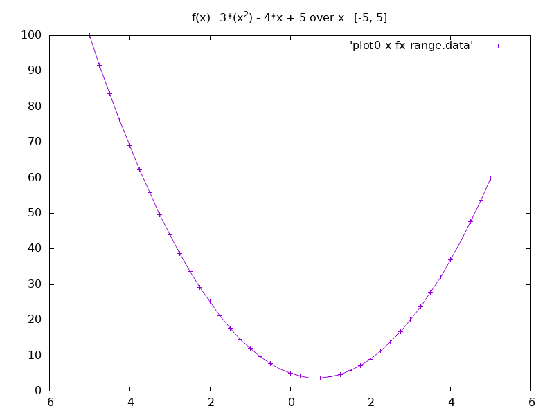
• Lets define a scalar valued function f(x), and get its value.

function f(x)
    return (3*(x^2)) - (4*x) + 5
end

f(3.0)
-- 20.0

• We can also plot this function over a range of values.

for x = -5, 5, 0.25 do
    print(x, f(x))
end

-- values plot given below

3.1. Derivative of the Expression

• Now we will think about the derivative of the expression.
• See the Differentiation rules
• In neural networks no one actually writes an expression and derives it.
• We are not going for the symbolic approach.
• We will try and understand what the derivative is measuring and what it is telling us about the function.
• We look at the definition of the derivative in terms of Limit from the wiki page of derivative. Derivative as a Limit.
• Basically how does the function respond to an infinitesimal change in the input variable. What is the slope of the function at the point.

-- if we use too small h, we will eventuall get an incorrect value because
-- we are using floating point arithmetic.
h = 0.00001
x = 3.0

f(x+h)
-- 20.014003

(f(x+h) - f(x))/h
-- 14.003000000002

• From the above we can conclude that at x=3 the slope of f(x) is 14.
• We can also calculate using the derivative of f(x).
• f'(x) or df(x)/dx = 6*x - 4
• Therefore f'(x) at x = 3 is 14.

3.2. Derivative at Another Point (x = -3)

• Let's calculate slope at another point, say x = -3
• Even looking at the plot we can see that the slope of the function at x = -3 is negative. Therefore the sign of the slope will be 'minus'.
• Slope or f'(-3) is -22.

x = -3

(f(x+h) - f(x))/h
-- -21.999970000053

3.3. Derivative goes to 0

• At x=2/3, the function's slope is 0.
• So the function will not respond to a nudge at this point.

x = 2/3

(f(x+h) - f(x))/h
-- 3.0000002482211e-05

4. Part 2: A More Complex Case

• Let's take a function with more than one inputs.
• We consider a function with three scalar inputs - a, b, c with a single output d.

a = 2.0
b = -3.0
c = 10.0

d = a*b + c

d
-- 4.0

• Now we would like to get the derivative of d w.r.t a, b and c.
• We would like to get the intuition of what this will look like.
• Lets start with derivative with respect to a. This means we will change a by a small amount and calculate d. And then we will calculate slope at the point.
• The value of d reduces by a small amount when we increase h by a small amount, as a is multiplied by b in the expression, and b is negative. Thus increase in a decreases the value of d.
• This gives us an intuition about the slope of d with respect to a.
• Note that using rules of differentiation also we will get the same answer as the calculation below.
• d(d)/da = b; therefore slope is b = -3.0

h = 0.00001
a = 2.0
b = -3.0
c = 10.0

d1 = a*b + c

a = a + h

d2 = a*b + c

print('d1 = ' .. d1)
-- d1 = 4.0
print('d2 = ' .. d2)
-- d2 = 3.99997
print('slope = ' .. (d2 - d1)/h)
-- slope = -3.0000000000641

• Now lets consider the derivative of d w.r.t. b.
• Again from the rules of differentiation d(d)/db = a.
• Therefore we should expect the answer 2.0.

h = 0.00001
a = 2.0
b = -3.0
c = 10.0

d1 = a*b + c

b = b + h

d2 = a*b + c

print('d1 = ' .. d1)
-- d1 = 4.0
print('d2 = ' .. d2)
-- d2 = 4.00002
print('slope = ' .. (d2 - d1)/h)
-- slope = 2.0000000000131

• Finally lets consider the derivative of d w.r.t. c.
• From the rules of differentiation d(d)/dc = 1.
• With changes in c, d changes by the exact same amount.

h = 0.00001
a = 2.0
b = -3.0
c = 10.0

d1 = a*b + c

c = c + h

d2 = a*b + c

print('d1 = ' .. d1)
-- d1 = 4.0
print('d2 = ' .. d2)
-- d2 = 4.00001
print('slope = ' .. (d2 - d1)/h)
-- slope = 0.99999999996214

• We have some intuitions about how expressions and their derivatives will work.
• Lets move to neural networks which will have massive expressions.

5. Part 3: Expressions for Neural Networks

As mentioned neural networks will have massive expressions. So we need some datastructure to maintain the massive expressions. And so we will build out the Value object which was shown in the beginning of the video, from the README of the micrograd project.

5.1. Core Value Object

• Lets start with the skeleton of a very simple value object.
• Lua Note: Lua is object-oriented but does not have classes. To keep the structure of the code similar to the one in the video, we will write the classes using the excellent middleclass library.
  • The code will be slightly more verbose than python.
• Here we create a simple value class, then create an instance a, and finally print it out.
• Lua Note: To make sure the code can be run in an interpreter, all Lua variables are being created in global scope. Usually we would write the code in files, and make sure that the variables are marked local.

class = require 'lib/middleclass'

-- Declare the class Value
Value = class('Value') -- 'Value' is the class' name

-- constructor
function Value:initialize(data)
  self.data = data
end

-- tostring
function Value:__tostring()
  return 'Value(data = ' .. self.data .. ')'
end

a = Value(2.0)

a
-- Value(data = 2.0)

5.2. Addition of Value Objects

• Now, we would like to create mutliple values and also be able to do things like a + b where a and b are values.
• We're going to use the metamethod __add in Lua to allow us to define addtion for Value objects.
• The addition inside Value:__add is a simple floating point addition of the data of two Value objects.

class = require 'lib/middleclass'

function Value:initialize(data)
  self.data = data
end

function Value:__tostring()
  return 'Value(data = ' .. self.data .. ')'
end

-- add this Value object with another
-- using metamethod _add
function Value:__add(other)
  return Value(self.data + other.data)
end

a = Value(2.0)
b = Value(-3.0)

-- this line will invoke the metamethod Value:__add
a + b
-- Value(data = -1.0)

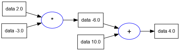
5.3. Multiplication of Value Objects

• Multiplication of Value objects is fairly simple and uses the __mul metamethod.
• This will now help us write expressions like a * b and a * b + c.

-- Class definition same as in the previous snippet.
-- multiply this Value object with another
-- using metamethod _mul
function Value:__mul(other)
  return Value(self.data * other.data)
end

a = Value(2.0)
b = Value(-3.0)
c = Value(10.0)

a * b
-- Value(data = -6.0)

-- the next line is equivalent to
-- (a.__mul(b)).__add(c)
d = a * b + c

d
--Value(data = 4.0)

5.4. Children of Value Objects

• What we're missing is the connective tissue of the expression.
• We want to keep these expression graphs, so we need to keep pointers about what values produce what other values.
• So we're going to introduce a new variable called _children which will be by default an empty tuple.
• Lua Note: Lua does not have tuples. In fact it has only one in-built compound datatype tables. So we're going to use a table to store _children.
• Internally the children are stored as set for efficiency.
• Lua Note: Lua does not have sets either. However sets can be eumulated in Lua using tables by keeping the elements as indices of a table. See 11.5 – Sets and Bags (Programming in Lua) for details of this approach.

class = require 'lib/middleclass'
Set = require 'util/set'

Value = class('Value')

function Value:initialize(data, _children)
  self.data = data
  if _children == nil then
    self._prev = Set.empty()
  else
    self._prev = Set(_children)
  end
end

function Value:__tostring()
  return 'Value(data = ' .. self.data .. ')'
end

function Value:__add(other)
  return Value(self.data + other.data, {self, other})
end

function Value:__mul(other)
  return Value(self.data * other.data, {self, other})
end

a = Value(2.0)
b = Value(-3.0)
c = Value(10.0)

d = a * b + c

d._prev
-- {Value(data = -6.0), Value(data = 10.0)}

5.5. Storing the Operation

• In addition to the children for a Value, we will also store the operation which was used to generate the Value.
• _op will be a private variable storing the operation as a string.

class = require 'lib/middleclass'
Set = require 'util/set'

Value = class('Value')

function Value:initialize(data, _children, _op)
  self.data = data
  self._op = _op or ''
  if _children == nil then
    self._prev = Set.empty()
  else
    self._prev = Set(_children)
  end
end

function Value:__tostring()
  return 'Value(data = ' .. self.data .. ')'
end

function Value:__add(other)
  return Value(self.data + other.data, {self, other}, '+')
end

function Value:__mul(other)
  return Value(self.data * other.data, {self, other}, '*')
end

a = Value(2.0)
b = Value(-3.0)
c = Value(10.0)

d = a * b + c
d._op
-- +

5.6. Visualizing the Expression Graph

• Since the expressions we write will get larger, Andrej introduces some code to generate a GraphViz plot of the expression graph, using a python libary.
• Lua Note: Since there is no cross-platform graphviz library available, I've implemented a small utility which calls the graphviz dot program with a temporary dot file and generates the graph in png format.

trace_graph = require("util/trace_graph")
trace_graph.draw_dot_png(d, "plots/plot1-graph_of_expr.png")

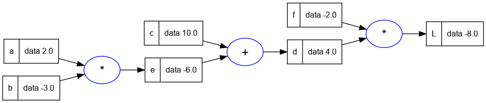
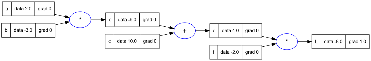
5.7. Label for Each Value Node in the Graph

• To improve the display of the expression graph, we will add a label to each node to help us identify the variable in at each node.
• We will also use a slightly larger expression this time.

class = require 'lib/middleclass'
Set = require 'util/set'

--- Declare the class Value
Value = class('Value')

--- static incrementing identifier
Value.static._next_id = 0

--- static method to get the next identifier
function Value.static.next_id()
    local next = Value.static._next_id
    Value.static._next_id = Value.static._next_id + 1
    return next
end

--- constructor
function Value:initialize(data, _children, _op, label)
    self.data = data
    self._op = _op or ''
    self.label = label or ''
    self.id = Value.next_id()
    if _children == nil then
        self._prev = Set.empty()
    else
        self._prev = Set(_children)
    end
end

--- string representation of the Value object
function Value:__tostring()
    return 'Value(data = ' .. self.data .. ')'
end

--- add this Value object with another
-- using metamethod _add
function Value:__add(other)
    return Value(self.data + other.data, { self, other }, '+')
end

--- multiply this Value object with another
-- using metamethod _mul
function Value:__mul(other)
    return Value(self.data * other.data, { self, other }, '*')
end

a = Value(2.0)
a.label = 'a'
b = Value(-3.0)
b.label = 'b'
c = Value(10.0)
c.label = 'c'

e = a * b
e.label = 'e'

d = e + c
d.label = 'd'

f = Value(-2.0)
f.label = 'f'

L = d * f
L.label = 'L'

-- print the graph
trace_graph = require("util/trace_graph")
trace_graph.draw_dot_png(L, "plots/plot2-expr_with_label.png")

5.8. Recap so far

• We're able to build out mathematical expressions with + and *.
• Expressions are scalar valued.
• We can do a forward pass and calculate the values at each node of the expression.
• We have inputs like a, b, c and output L.
• We can visualize the forward pass in a graph.

Next Steps: We're going to start at the end of the expression (the output) and calculate the gradient/derivative of each output w.r.t each node. This is called back-propagation. So in the example above we will calculate dL/dL, dL/df, dL/dd etc.

In the neural network setting we're very interested in the derivative of the loss function L w.r.t the weights of the neural network. So for now there are these internal nodes, which will eventually be the weights of a neural network. And we will need to know how those weights are impacting the loss function.

We will usually not be interested in the derivative of the loss function w.r.t the input data nodes, because the data is fixed. We will iterate upon the weights of the neural network.

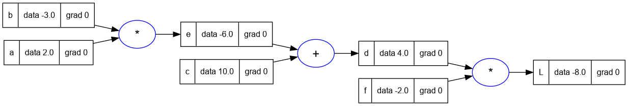
So in the next steps we will change the Value class to maintain the derivative of the loss w.r.t to this value. And this member of the Value class will be called grad. The value of grad initial will be 0, which means no effect. At initialization we assume every value does not impact the output/loss. Changing this variable does not change the loss.

--- constructor
function Value:initialize(data, _children, _op, label)
    self.data = data
    self.grad = 0
    self._op = _op or ''
    self.label = label or ''
    self.id = Value.next_id()
    if _children == nil then
        self._prev = Set.empty()
    else
        self._prev = Set(_children)
    end
end

a = Value(2.0)
a.label = 'a'
b = Value(-3.0)
b.label = 'b'
c = Value(10.0)
c.label = 'c'

e = a * b
e.label = 'e'

d = e + c
d.label = 'd'

f = Value(-2.0)
f.label = 'f'

L = d * f
L.label = 'L'

trace_graph.draw_dot_png(L, "plots/plot3-with_grad.png")

6. Part 4: Manual Back-propagation of an Expression

• We can start with L in the expression above. And calculate the derivative of L w.r.t L, which will be one. This can also be demonstrated by calculating ((L + h) - L) / h, which will be h/h i.e. 1.
• Now we can write a function to calculate the derivative of L w.r.t the other Values and write them down.

function lol()
  local a, b, c, d, e, f, L
  local h = 0.001

  a = Value(2.0)
  a.label = 'a'
  b = Value(-3.0)
  b.label = 'b'
  c = Value(10.0)
  c.label = 'c'
  e = a * b
  e.label = 'e'
  d = e + c
  d.label = 'd'
  f = Value(-2.0)
  f.label = 'f'
  L = d * f
  L.label = 'L'
  local L1 = L.data

  a = Value(2.0)
  a.label = 'a'
  b = Value(-3.0)
  b.label = 'b'
  c = Value(10.0)
  c.label = 'c'
  e = a * b
  e.label = 'e'
  d = e + c
  d.label = 'd'
  f = Value(-2.0)
  f.label = 'f'
  L = d * f
  L.label = 'L'
  local L2 = L.data + h

  print((L2 - L1)/h)
end

lol()
-- 1.0000000000003

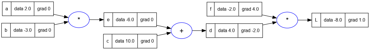
• Now let's set dL/dL to 1.0 and redraw the graph

L.grad = 1.0
trace_graph.draw_dot_png(L, "plots/plot4-L_grad.png")

• Now let's calculate dL/df and dL/dd.
• since L = f * d, then by rules of differentiation we have
• dL/df = d = 4.0, and
• dL/dd = f = -2.0
• We can also modify the above function to apply +h to d and f in turn to calculate this programmatically.

d.grad = -2.0
f.grad = 4.0
trace_graph.draw_dot_png(L, "plots/plot5-f_and_d_grad.png")

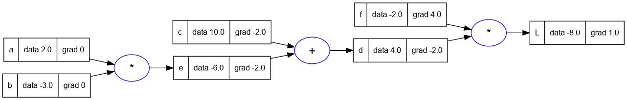
• Now going back in the network let's calculate dL/dc and dL/de.
• Here we will use the rule that df/dx = df/dy * dy/dx. This is the chain rule of calculus.
• See the Intuitive explanation of the chain rule.
• Since dL/dd is known then if we can calculate dd/dc then we can get dL/dc = dL/dd * dd/dc.
• We can use similar reasoning for dL/de.
• dd/dc and dd/de are local gradients.
• Given d = c + e, as we can see from the expression, dd/dc = 1.0 and also dd/de = 1.0.
• And so dL/dc = dL/dd * dd/dc = -2.0 * 1.0 = -2.0.
• And dL/de = dL/dd * dd/de = -2.0 * 1.0 = -2.0.

c.grad = -2.0
e.grad = -2.0
trace_graph.draw_dot_png(L, "plots/plot6-c_and_e_grad.png")

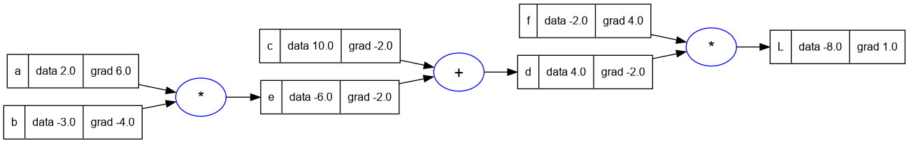
• We have one more layer remaining to go back to.
• Lets calculate the gradient for a and b.
• We will apply the chain rule again.
• Since e = a * b, de/db = a and de/da = b.
• Since dL/de = -2.0 and de/da = b = -3.0, therefore dL/da = dL/de * de/da = -2.0 * -3.0 = 6.0
• Similarly dL/db = dL/de * de/db = -2.0 * a = -2.0 * 2.0 = -4.0.

a.grad = 6.0
b.grad = -4.0
trace_graph.draw_dot_png(L, "plots/plot7-a_and_b_grad.png")

Note: At each step above, Andrej also modifies the function lol() and verifies the derivative value programmatically. I haven't repeated the code as it is self explanatory but quite verbose.

• At this point we can consider what back-propagation is, it is the multiplying the derivatives backward through the expression graph by applying the chain rule, till we reach the leaf nodes, and all nodes have their gradient/ derivative applied.

7. Part 5: Single Optimization Step: Nudge Inputs to Change Loss

• Now that we know the gradients at each input, we can verify that when we change the inputs by a small amount nudge it, then we can creat a small change in the L.

a.data = a.data + (0.01 * a.grad)
b.data = b.data + (0.01 * b.grad)
c.data = c.data + (0.01 * c.grad)
d.data = d.data + (0.01 * d.grad)
e = a * b
d = e + c
L = d * f
L.data
-- -7.4352

8. Part 6: Manual Back-propagation of a Single Neuron

• We're going to do a more useful example of manual backpropagation, for a neuron.
• Andrej refers to an image of a neuron in his video which is from the course notes of CS231n: Convolutional Neural Networks for Visual Recognition.
• He also refers to an image of two-layer neural net - multi-layer perceptrons from the same course notes.
• I've included both the images below for reference.

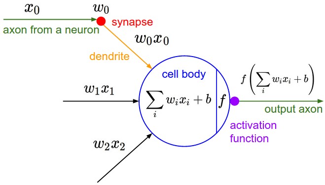
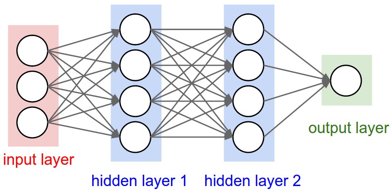
Salient Points * The two-layer networks contains multiple neurons connected to each other. * Biologically, neurons are complicated. * We have simple mathematical representations/models of them. * The image of the single neuron above has the following: * Inputs - some input data, there are multiple inputs say xi, where i is a number. * Synapses - connecting input data to neuron, that have weights in them. The wi are weights. What flows to the cell body are the multiplication of synapse weights with the inputs i.e. wi * xi. * Bias - the cell body has some bias b. This is the innate trigger-happiness(sic) of the neuron. It is added to the sum of the weighted inputs of the neuron. * Activation Function - the weight sum plus bias of the cell are taken through an activation function. This activation function is usually some kind of a squashing function(sic) - like a sigmoid, or tanh or similar.

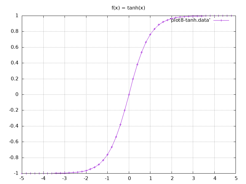
8.1. The tanh function

• We're going to use the tanh for our activation function.
• Lua Note: Lua does not have tanh function, so I've implemented a simple version in the util/tanh.lua.

tanh = require('util/tanh')

datfile = io.open('plots/plot8-tanh.data', 'w')

--- print x and tanh(x) as a table
for x = -5, 5, 0.2 do
  print(x .. ' ' .. tanh(x))
  datfile:write(x .. ' ' .. tanh(x) .. '\n')
end

datfile:close()

-- -5.0 -0.9999092042626
-- -4.8 -0.99986455170076
-- -4.6 -0.99979794161218
-- output snipped

• Here is the gnuplot script to plot the data, followed by the plot.
• Salient Points:
• The input as it comes in, the output gets squashed initially.
• As the input grows output starts rising quite fast and at some point starts rising linearly.
• Finally at a particular value the function starts to plateau again, and then the increase almost stops completely.
• Input as it comes in we're going to cap it smoothly at 1, and at the negative side we're going to cap it smoothly to -1.

# Image output of size 800x600
set terminal png size 800,600
# Output file name
set output 'plot8.png'
# Plot title
set title 'f(x) = tanh(x)'
# Set the grid
set grid
# Plot the data
plot 'plot8-tanh.data' with linespoints

• So finally what comes out of the neuron is the weighted sum of inputs $$w_i x_i$$, plus a bias b, squashed by an activation function f.

$$ f \left( \sum_i w_i x_i + b\right) $$

8.2. tanh support in Value class

• Before we can use the tanh function we need to add support for this in our Value class.
• Here's what the implementation looks like...

function Value:tanh()
    local x = self.data
    local t = (math.exp(2 * x) - 1)/(math.exp(2 * x) + 1)
    return Value(t, { self }, 'tanh')
end

8.3. Expression for a Neuron

• let's create a neuron expression with inputs, weights, bias and activation function now.

-- inputs x1, x2
x1 = Value(2.0); x1.label = 'x1'
x2 = Value(0.0); x2.label = 'x2'
-- weights w1, w2
w1 = Value(-3.0); w1.label = 'w1'
w2 = Value(1.0); w2.label = 'w2'
-- bias of the neuron
b = Value(6.7); b.label = 'b'
x1w1 = x1 * w1; x1w1.label = 'x1w1'
x2w2 = x2 * w2; x2w2.label = 'x2w2'
x1w1x2w2 = x1w1 + x2w2; x1w1x2w2.label = 'x1w1 + x2w2'
n = x1w1x2w2 + b; n.label = 'n'
o = n:tanh(); o.label = 'o'

-- print the graph
trace_graph = require("util/trace_graph")
trace_graph.draw_dot_png(o, "plots/plot9-neuron_expr.png")

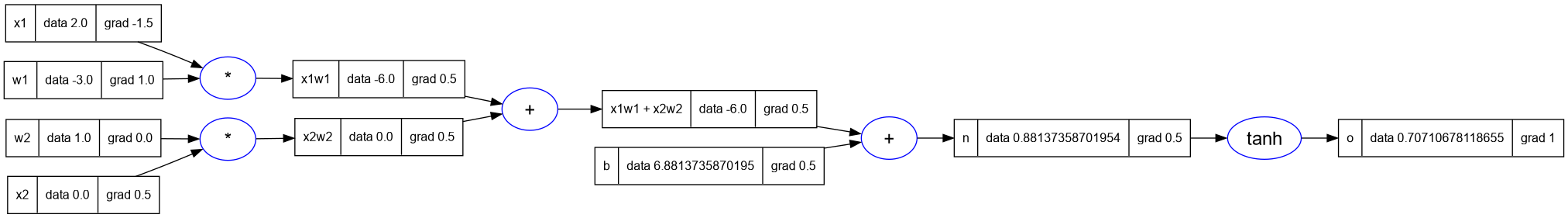
8.4. Backpropagation on a Neuron

• Andrej sets some specific value of bias, in the previous expression, so that gradients will be easier to calculate.
• Lets set the same values here:

-- inputs x1, x2
x1 = Value(2.0); x1.label = 'x1'
x2 = Value(0.0); x2.label = 'x2'
-- weights w1, w2
w1 = Value(-3.0); w1.label = 'w1'
w2 = Value(1.0); w2.label = 'w2'
-- bias of the neuron
b = Value(6.8813735870195432); b.label = 'b'
x1w1 = x1 * w1; x1w1.label = 'x1w1'
x2w2 = x2 * w2; x2w2.label = 'x2w2'
x1w1x2w2 = x1w1 + x2w2; x1w1x2w2.label = 'x1w1 + x2w2'
n = x1w1x2w2 + b; n.label = 'n'
o = n:tanh(); o.label = 'o'

-- print the graph
trace_graph = require("util/trace_graph")
trace_graph.draw_dot_png(o, "plots/plot10-neuron_b_changed.png")

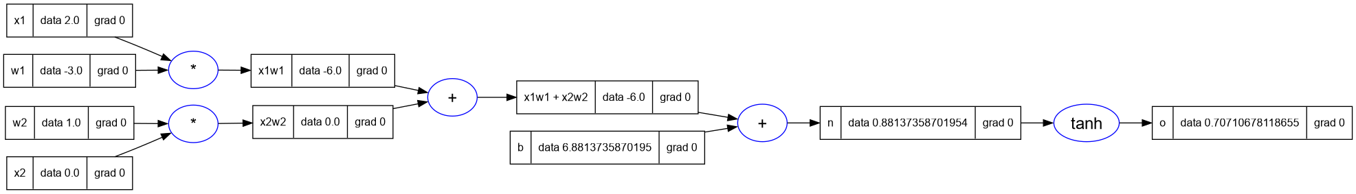
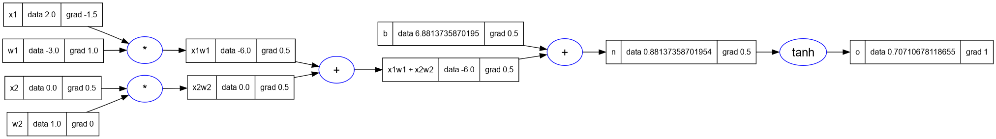
• Lets start out with o, the output node. What is do/do. The base case, it is 1.

o.grad = 1

• To calculate do/dn, where o = tanh(n) we need to know the derivative of tanh.
• Derivative of tanh is 1 - tanh^2(x).
• So do/dn = 1 - (tanh(n) ** 2) = 1 - o**2

n.grad = 1 - (o.data ^ 2)
n.grad
-- 0.5

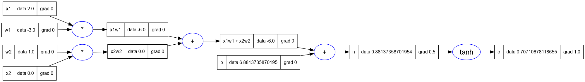
• Lets go one more level back.
• And we have a plus operation. We know from earlier in our expression analysis that + is just a distributor of the gradient.

x1w1x2w2.grad = n.grad
b.grad = n.grad

• We have another plus next, so we will distribute the gradient again.

x2w2.grad = x1w1x2w2.grad
x1w1.grad = x1w1x2w2.grad

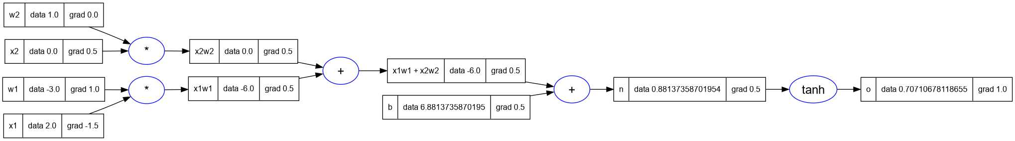
• The next two are * nodes. In a multiple/times node, we know that the local derivative of one term is the other term multiplied with the gradient of the result.
• So setting these we have...

x2.grad = w2.data * x2w2.grad
w2.grad = x2.data * x2d2.grad
x1.grad = w1.data * x1w1.grad
w1.grad = x1.data * x1w1.grad

trace_graph.draw_dot_png(o, "plots/plot11-neuron_with_grads.png")

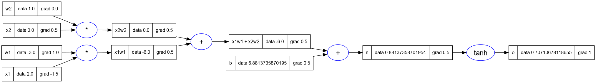
• Notice that since x2 = 0, therefore the gradient of its weight w2.grad = 0
• This is according to our intuition, because the input is zero, so the result does not impact the next node.
• So these are the final derivatives.

9. Part 7: Backpropagation Implementation

• Now that we know how gradients can be calculated manually in the expression graph, we can start to implement this backpropagation of gradients in the Value class.
• We will now have _backward a member of the Value class which will help us chain the output gradient to the input gradient.
• By default this will be a function which will do nothing. In micrograd python version this is written as _backward = lambda: None.
• This empty function will be the case for for e.g. the leaf node. For a leaf node there is nothing to backpropagate.
• But when we are creating a Value using one of the supported operations, we would be creating new Value objects.
• Then we will have to define the current Value objects gradient.
• The idea is to propagate the output's gradient to self's gradient and other's gradient in some way. And how it is propagated is different for each supported operation
• The pseudocode looks like

function _backward()
  self.grad = ???
  other.grad = ???
end

out._backward = _backward

9.1. _backward function for __add

• For e.g. for the add operation self._grad = 1.0 * out.grad, and similarly other._grad = 1.0 * out.grad.
• Therefore the newly created _backward can be called after all forward pass expression calculations are completed.

9.2. _backward function for __mul

function _backward()
  self.grad = other.grad * out.grad
  other.grad = self.grad * out.grad
end

out._backward = _backward

9.3. _backward function for tanh

function _backward()
  self.grad = (1 - t**2) * out.grad
end

out._backward = _backwa()

9.4. Redoing the backpropagation on the expression using _backward

• We will use the _backward function on the output node to backpropagate the gradients back through the expression graph.
• Notice that the grad is set to 0 by default for every Value node.
• Therefore we will set the grad of the output node o to 1.0 before we start the backpropagation.

Value = require('nanograd/engine')

-- inputs x1, x2
x1 = Value(2.0); x1.label = 'x1'
x2 = Value(0.0); x2.label = 'x2'
-- weights w1, w2
w1 = Value(-3.0); w1.label = 'w1'
w2 = Value(1.0); w2.label = 'w2'
-- bias of the neuron
b = Value(6.8813735870195432); b.label = 'b'
x1w1 = x1 * w1; x1w1.label = 'x1w1'
x2w2 = x2 * w2; x2w2.label = 'x2w2'
x1w1x2w2 = x1w1 + x2w2; x1w1x2w2.label = 'x1w1 + x2w2'
n = x1w1x2w2 + b; n.label = 'n'
o = n:tanh(); o.label = 'o'

-- set the grad of o to 1.0
o.grad = 1.0

-- backpropagate using _backward
o._backward()

-- print the graph
trace_graph = require("util/trace_graph")
trace_graph.draw_dot_png(o, "plots/plot12-o_backprop.png")

• Now let's call the _backward on n which is the next Value node going backward in the expression graph.
• And then we will call _backward on b, which if you notice is a leaf node.
• And then we will call _backward on x1w1x2w2, followed by x1w1 and x2w2.
• Let's make these calls and look at the results

n._backward()
b._backward()
x1w1x2w2._backward()
x1w1._backward()
x2w2._backward()

-- print the graph
trace_graph = require("util/trace_graph")
trace_graph.draw_dot_png(o, "plots/plot13-all_backprop.png")

• Notice that the results are exactly as we had before in the manual back- propagation. But now we have done it through the automatic calcualation.

10. Part 8: Backpropagation for the entire expression graph

• When we do the backpropagation by calling the _backward function manually we're laying out the expression graph and calling the function starting from the output node and going left-wards (backwards) in the graph.
• And we cannot initial the backpropagation of the output node unless all the values in the expressions have been calculated upto the output node.
• All the dependencies of a node should have been calculated before we can call _backward on it.
• The way we achieve this by doing something called Topological Sort.
• Topological Sort is the laying out of a graph such that all the edges are going in one direction say left-to-right.
• Andrej suggests reading more about the topic, but simply provides an implementation for the sort in python.
• And here I've implemented the same code in lua.

Set = require('util/Set')
topo = {}
visited = Set.empty()

function build_topo(v)
  if not visited:contains(v) then
    visited:add(v)
    for _, child in ipairs(v._prev:items()) do
      build_topo(child)
    end
    table.insert(topo, v)
  end
end

build_topo(o)
for _, v in ipairs(topo) do print(v) end

-- Value(data = 2.0)
-- Value(data = -3.0)
-- Value(data = -6.0)
-- Value(data = 0.0)
-- Value(data = 1.0)
-- Value(data = 0.0)
-- Value(data = -6.0)
-- Value(data = 6.8813735870195)
-- Value(data = 0.88137358701954)
-- Value(data = 0.70710678118655)

• Now let's use the topological sort to do what we did manually.
• We will set the gradient of the output node as 1.
• Then we will call the _backward function on each Value node in the topo sort (but in the reverse order).

o.grad = 1
for i = #topo, 1, -1 do
    topo[i]._backward()
end

-- print the graph
trace_graph = require("util/trace_graph")
trace_graph.draw_dot_png(o, "plots/plot14-using_topo_sort.png")

10.1. Implement the backward function in Value class

• Now we will move this backward function into the Value class like so...

--- implement the backpropagation for the Value
function Value:backward()
    local topo = {}
    local visited = Set.empty()

    local function build_topo(v)
      if not visited:contains(v) then
        visited:add(v)
        for _, child in ipairs(v._prev:items()) do
          build_topo(child)
        end
        table.insert(topo, v)
      end
    end

    build_topo(self)

    -- visit each node in the topological sort (in the reverse order)
    -- and call the _backward function on each Value
    self.grad = 1
    for i = #topo, 1, -1 do
        topo[i]._backward()
    end
end

• And finally we can just setup the neuron expression and call o.backward to get the gradients.

Value = require('nanograd/engine')

-- inputs x1, x2
x1 = Value(2.0); x1.label = 'x1'
x2 = Value(0.0); x2.label = 'x2'
-- weights w1, w2
w1 = Value(-3.0); w1.label = 'w1'
w2 = Value(1.0); w2.label = 'w2'
-- bias of the neuron
b = Value(6.8813735870195432); b.label = 'b'
x1w1 = x1 * w1; x1w1.label = 'x1w1'
x2w2 = x2 * w2; x2w2.label = 'x2w2'
x1w1x2w2 = x1w1 + x2w2; x1w1x2w2.label = 'x1w1 + x2w2'
n = x1w1x2w2 + b; n.label = 'n'
o = n:tanh(); o.label = 'o'

-- backpropagation
o:backward()

-- print the graph
trace_graph = require("util/trace_graph")
trace_graph.draw_dot_png(o, "plots/plot15-o_backprop_using_backward.png")

11. Part 9: Fixing backprop bug when using a node multiple times.

• We have a bug in the existing implemetation of backpropagation which only surfaces in certain cases.
• If we reuse the same node multiple times in the expression, it's gradient is calculated incorrectly.
• And this incorrect value is propagated through the rest of the graph.
• Here's an example of the bug.

Value = require('nanograd/engine')

a = Value(3.0); a.label = 'a'
b = a + a; b.label = 'b'
b:backward()

trace_graph = require("util/trace_graph")
trace_graph.draw_dot_png(b, "plots/plot16-backprop_bug_1.png")

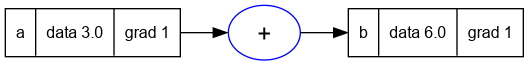
• There are two a nodes in the graph above but they are on top of another.
• And notice the gradients calculated for a and b.
• The grad for b is correctly set to 1.
• However since b = f(a) = 2 * a, therefore f'(a) = db/da = 2.
• But the grad of a is incorrectly marked 1.
• Now this occurs because of these two lines in the _add function of Value

  self.grad = 1 * out.grad
  other.grad = 1 * out.grad

• Even though in the case of b = a + a, both self and other are the same node, notice that their grads are overwritten by the two lines to 1.

11.1. A longer expression

• Lets use a longer more complicated expression to demonstrate the bug.

a = Value(-2.0); a.label = 'a'
b = Value(3.0); b.label = 'b'

d = a * b; d.label = 'd'
e = a + b; e.label = 'e'
f = d * e; f.label = 'f'

f:backward()

trace_graph.draw_dot_png(f, "plots/plot17-backprop_bug_2.png")

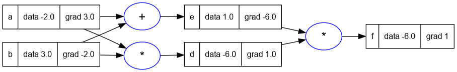
• You can see that the a and b nodes are used more than once in this expression.
• And this graph also has the same issue as the expression in the previous example.
• While backpropagating, we will visit b and a more than once, and each time their grad value will be overwritten. Thus resulting in incorrect values.

11.2. Solution for the bug

• We need to fix the overwriting of the gradients.
• See the "Multivariable chain rule", we need to accumulate the gradients using addition instead of replacing them.
• Therefore the solution to the bug is simple, we need to change the two lines which replace self.grad and other.grad to accumulate instead of replace values.

  self.grad = self.grad + (1 * out.grad)
  other.grad = other.grad + (1 * out.grad)

• We need to make these changes/fixes in every _backward internal function, and then we have the gradients accumulated correctly.

--- Declare the class Value
Value = class('Value')

--- static incrementing identifier
Value.static._next_id = 0

--- static method to get the next identifier
function Value.static.next_id()
    local next = Value.static._next_id
    Value.static._next_id = Value.static._next_id + 1
    return next
end

--- constructor
function Value:initialize(data, _children, _op, label)
    self.data = data
    self.grad = 0
    self._op = _op or ''
    self.label = label or ''
    self._backward = function() end
    self.id = Value.next_id()
    if _children == nil then
        self._prev = Set.empty()
    else
        self._prev = Set(_children)
    end
end

--- string representation of the Value object
function Value:__tostring()
    return 'Value(data = ' .. self.data .. ')'
end

--- add this Value object with another
-- using metamethod _add
function Value:__add(other)
    local out = Value(self.data + other.data, { self, other }, '+')
    local _backward = function()
        self.grad = self.grad + (1 * out.grad)
        other.grad = other.grad + (1 * out.grad)
    end
    out._backward = _backward
    return out
end

--- multiply this Value object with another
-- using metamethod _mul
function Value:__mul(other)
    local out = Value(self.data * other.data, { self, other }, '*')
    local _backward = function()
        self.grad = self.grad + (other.data * out.grad)
        other.grad = other.grad + (self.data * out.grad)
    end
    out._backward = _backward
    return out
end

--- implement the tanh function for the Value class
function Value:tanh()
    local x = self.data
    local t = (math.exp(2 * x) - 1) / (math.exp(2 * x) + 1)
    local out = Value(t, { self }, 'tanh')
    local _backward = function()
        self.grad = self.grad + ((1 - t * t) * out.grad)
    end
    out._backward = _backward
    return out
end

--- implement the backpropagation for the Value
function Value:backward()
    local topo = {}
    local visited = Set.empty()

    local function build_topo(v)
        if not visited:contains(v) then
            visited:add(v)
            for _, child in ipairs(v._prev:items()) do
                build_topo(child)
            end
            table.insert(topo, v)
        end
    end

    build_topo(self)

    -- visit each node in the topological sort (in the reverse order)
    -- and call the _backward function on each Value
    self.grad = 1
    for i = #topo, 1, -1 do
        topo[i]._backward()
    end
end

11.3. Examples fixed

• We can run the previous examples and see that the bug is now fixed.

Value = require('nanograd/engine')

a = Value(3.0); a.label = 'a'
b = a + a; b.label = 'b'
b:backward()

trace_graph = require("util/trace_graph")
trace_graph.draw_dot_png(b, "plots/plot18-fixed_example1.png")

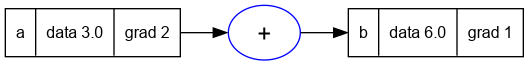
• We can see in the graph above that the gradient at a is now correctly set to 2.
• Similarly for the longer expression in the previous section.

a = Value(-2.0); a.label = 'a'
b = Value(3.0); b.label = 'b'

d = a * b; d.label = 'd'
e = a + b; e.label = 'e'
f = d * e; f.label = 'f'

f:backward()

trace_graph.draw_dot_png(f, "plots/plot19-fixed_example2.png")

12. Part 10: Breaking up tanh: Adding more operations to Value

• In this part of the video Andrej goes on to implement more operations in the Value class.
• One of the goals is to expand the tanh function and implement its formula.
• This is a sort of repetition of the concepts considered in the previous sections and reinforces the learnings.
• The first operation we add support for is adding Value objects to constants.

12.1. Supporting constants in Value.__add

• Andrej adds support for this in the __add__ metamethod using the check for the type of other using the instanceof operator.
• In lua I've implemented this slightly differently, by checking if the type of other is number and in that case creating a Value
• In lua the same method is used by the runtime, when the order of operations is reversed (solved in python using the __rmul__ method).
• Therefore in lua I have to handle the additional situation when self is a number. To not pollute the global self, I've used a local this variable to create a new Value object when self is a number.

function Value:__add(other)
    local this = self
    if type(other) == 'number' then
        other = Value(other)
    end
    if type(self) == 'number' then
        this = Value(self)
    end

    local out = Value(this.data + other.data, { this, other }, '+')
    local _backward = function()
        this.grad = this.grad + (1 * out.grad)
        other.grad = other.grad + (1 * out.grad)
    end
    out._backward = _backward
    return out
end

• Once the above changes are done in the Value class we can write.

Value = require('nanograd/engine')

2 + Value(2)
-- Value(data = 4)

Value(2) + 2
-- Value(data = 4)

12.2. Adding support for exponentiation in Value

• We now add support for exponentiation in the Value class. This is required because one of the ways tanh can be implemented is by using the formula which expresses it in terms of the exponential function. See Exponential Definitions of Hyperbolic Functions

function Value:exp()
    local x = self.data
    local out = Value(math.exp(x), { self }, 'exp')
    local _backward = function()
        -- because the derivative of exp(x) is exp(x)
        -- and out.data = exp(x)
        self.grad = self.grad + (out.data * out.grad)
    end
    out._backward = _backward
    return out
end

• Here's an example of the exp function in a sample expression below.

Value = require('nanograd/engine')

a = Value(2.0)
a:exp()
-- Value(data = 7.3890560989307)

12.3. Adding support for division and subtraction

• Division and subtraction are the last two operations needed to be able to express the tanh function using exponentiation.
• Andrej demonstrates how to implement division in a more general form.
• We take into consideration the fact that a/b = a * 1/b = a * (b**-1).

• So we implement the power function which helps us implement division.

• First we implement subtraction in terms of negation, which is built upon multiplication with -1.

function Value:__unm()
    return self * -1
end

--- subtract this Value object with another
-- using metamethod _sub
function Value:__sub(other)
    return self + (-other)
end

• Here's an example

a = Value(2.0)
b = Value(4.0)
a - b
-- Value(data = -2.0)

• Here's how we implemented division using an implemetation of power.

function Value:__div(other)
    return self * other ^ -1
end

--- This is the power function for the Value class
-- using metamethod _pow
-- it does not support the case where the exponent is a Value
function Value:__pow(other)
    local this = self
    if type(other) ~= 'number' then
        error('Value:__pow: other must be a number')
    end

    if type(self) == 'number' then
        this = Value(self)
    end

    local out = Value(this.data ^ other, { this }, '^' .. other)
    local _backward = function()
        this.grad = this.grad
            + (other * (this.data ^ (other - 1)) * out.grad)
    end
    out._backward = _backward
    return out
end

12.4. Sample expression with tanh expanded

• Here's the expression with the tanh node expanded into its component parts.

Value = require('nanograd/engine')

-- inputs x1, x2
x1 = Value(2.0); x1.label = 'x1'
x2 = Value(0.0); x2.label = 'x2'
-- weights w1, w2
w1 = Value(-3.0); w1.label = 'w1'
w2 = Value(1.0); w2.label = 'w2'
-- bias of the neuron
b = Value(6.8813735870195432); b.label = 'b'
x1w1 = x1 * w1; x1w1.label = 'x1w1'
x2w2 = x2 * w2; x2w2.label = 'x2w2'
x1w1x2w2 = x1w1 + x2w2; x1w1x2w2.label = 'x1w1 + x2w2'
n = x1w1x2w2 + b; n.label = 'n'
e = (2 * n):exp(); e.label = 'e'
o = (e - 1)/(e + 1); o.label = 'o'

-- backpropagation
o:backward()

-- print the graph
trace_graph = require("util/trace_graph")
trace_graph.draw_dot_png(o, "plots/plot20-tanh_expanded.png")

• The above graph agrees with the previous non-expanded version of the expression in the previous sections.
• This shows two things:
• One: that these two expressions are equivalent
• Two: that the granularity of functions supported in the Value node is entirely up to us.
• As long as we can do the forward pass and backward pass of an operation, it does not matter what the operation is.

13. Part 11: The same example in PyTorch

• In this section of the video Andrej goes over how the same expression is implemented in PyTorch.
• He also explains that micrograd is a very simplified version of the operations in PyTorch.
• This section of the video begins around 1H35M, and I will not repeat the whole thing here.
• An example of PyTorch usage is also provided in the tests for micrograd.

14. Part 12: Building a neural net library (multi-layer perceptron)

• We have created a mechanism to create quite complex expression.
• And now we can use this mechanism to create neurons and then layers of neurons eventually leading up to neural networks.
• As neural networks are just a special class of mathematical expressions.
• So we will build a neural net piece by piece, and eventually we will build a 'two layer multi-layer perceptron'.
• Lets start with a single neuron.
• We will build a neuron that subscribes to the PyTorch API.
• Just like we matched the PyTorch API on the backprop side, we will try to do the same on the neural network.

class = require 'lib/middleclass'
Value = require 'nanograd/engine'

Neuron = class('Neuron')

--- constructor of a Neuron
-- @param nin number of inputs
function Neuron:initialize(nin)
    --- create a random number in the range [-1, 1]
    local function rand_float()
        return (math.random() - 0.5) * 2
    end

    -- create a table of random weights
    self.w = {}
    for _ = 1, nin do
        table.insert(self.w, Value(rand_float()))
    end

    -- create a random bias
    self.b = Value(rand_float())
end

--- forward pass of the Neuron
-- calculate the activation and then apply the activation function
-- which in our case is the tanh function
-- @param x input vector
function Neuron:__call(x)
    local act = self.b
    for i = 1, #self.w do
        act = act + self.w[i] * x[i]
    end
    local out = act:tanh()
    return out
end

x = {2.0, 3.0}
n = Neuron(2)
n(x)
-- Expected output: A Value object with value in the range [-1, 1]

14.1. Multi-layer perceptron

• Andrej again refers to the schematic of the mlp (multi-layered perceptron) from the course page of CS231n.
• He talks about hidden layer 1, and how there are several neurons in the layer and they are not connected to each other but they are fully connected to the inputs.

• So what is a layer of neurons, it's just a set of neurons evaluated independently.

Layer = class('Layer')

--- constructor of a Layer
-- @param nin number of inputs
-- @param nout number of outputs
function Layer:initialize(nin, nout)
    self.neurons = {}
    for _ = 1, nout do
        table.insert(self.neurons, Neuron(nin))
    end
end

--- forward pass of the Layer
-- @param x input vector
function Layer:__call(x)
    local outs = {}
    for _, neuron in ipairs(self.neurons) do
        table.insert(outs, neuron(x))
    end
    return outs
end

n = Layer(2, 3)
x = { Value(1), Value(2) }
y = n(x)
for _, v in ipairs(y) do
    print(v)
end
-- Expected output: A table of Value objects with value in the range [-1, 1]

14.2. Complete MLP

• Finally we complete the picture shown above and create a complete multi- -layer perceptron aka MLP.
• The multi-layer perceptron takes a number of inputs, and a list of numbers signifying the number of neurons in each layer.
• Below we try to replicate the sample mlp in the picture at the beginning of this section by create an mlp with 3 inputs, and 2 layers of 4 neurons each, and 1 output.

MLP = class('MLP')

--- constructor of a Multi-Layer Perceptron
function MLP:initialize(nin, nouts)
    local sz = table.pack(nin, table.unpack(nouts))
    self.layers = {}
    for i = 1, #nouts do
        table.insert(self.layers, Layer(sz[i], sz[i + 1]))
    end
end

--- forward pass of the MLP
-- @param x input vector
function MLP:__call(x)
    local out = x
    for _, layer in ipairs(self.layers) do
        out = layer(out)
    end
    return out
end

x = {2, 3, -1}
mlp = MLP(3, { 4, 4, 1 })
y = mlp(x)
for _, v in ipairs(y) do
    print(v)
end
-- Value(data = 0.31997025487794)
-- Expected output: A table of 1 Value object with value in the range [-1, 1]

• To make the above tabular output a little nicer, we make a change in Layer.__call to return only the first element if the number of outputs is exactly one.
• This helps us directly print out the result as one value instead of indexing it in a table whose length we know is 1.

--- forward pass of the Layer
-- @param x input vector
function Layer:__call(x)
    local outs = {}
    for _, neuron in ipairs(self.neurons) do
        table.insert(outs, neuron(x))
    end
    if #outs == 1 then
        return outs[1]
    end
    return outs
end

• And now to use it

nn = require('nanograd/nn')

x = {2, 3, -1}
n = nn.MLP(3, { 4, 4, 1 })
y = n(x)
y
-- Value(data = 0.21260160250202
-- Expected a value with value in range [-1, 1]

• We can plot the expression for the MLP, and you can see that the graph is quite complicated and large.
• "Open the image in a new window/top" and zoom-in to see the details.
• And we will be able to backpropagate through the expression using our backpropagation implementation.

trace_graph = require("util/trace_graph")
trace_graph.draw_dot_png(y, "plots/plot21-mlp.png")

15. Part 13: Working with a tiny dataset, writing a loss function

• We will start with a small example dataset created by Andrej.
• This dataset has four sets of 3 inputs each.
• And it also had the desired output for each of the four input sets.
• The expected output for xs[1] is ys[1] and so on.
• Lua Note: Array indexes in Lua are 1-based.
• This is basically a very simple binary classifier neural network that we would like to build here.

xs = {
  {2.0, 3.0, -1.0},
  {3.0, -1.0, 0.5},
  {0.5, 1.0, 1.0},
  {1.0, 1.0, -1.0},
}

ys = {1.0, -1.0, -1.0, 1.0} -- desired targets

• Let's see what values our neural network creates for these inputsAnd in
• We will create a set of neurons for each input set

-- get the predictions from our neural network
ypred = {}
for _, x in ipairs(xs) do
  table.insert(ypred, n(x))
end

-- print the predictions
for _, yval in ipairs(ypred) do
  print(yval)
end

-- Value(data = -0.2125230539818)
-- Value(data = -0.74155205138326)
-- Value(data = -0.11718987980605)
-- Value(data = -0.56119517054583)

• Notice that the values we get aren't the ones that we want.
• So how do we tune the neural net, how to set the weights to better predict the expected values.
• The trick used in deep learning is to calculate a single number which represents the performance of your entire neural network.
• We call this single number the loss.
• The loss is defined in such a way as to measure close we are to the expected values.
• And in our case we notice that the output values are quite far apart from th expected values so the loss is going to be high.
• So particularly in this example we're going to implement the Mean-squared error loss function.
• Lets calculate the squared-difference of each expected output and calculated output.
• The difference is small when the predicted output is close to the expected one and higher when it is not.
• Squaring the difference ensures that we are removing the sign of the difference, as we are only interested in the magnitude of the difference.
• We could also have taken an absolute value instead of a square.

for idx, ygt in ipairs(ys) do
  local yout = ypred[idx]
  local diff_sq = (yout - ygt) ^ 2
  print(diff_sq)
end

-- Value(data = 1.4702121564374)
-- Value(data = 0.0667953421442)
-- Value(data = 0.77935370831686)
-- Value(data = 2.4373303605356)

• The final loss is just the sum of all these squared difference values.

loss = 0
for idx, ygt in ipairs(ys) do
  local yout = ypred[idx]
  local diff_sq = (yout - ygt) ^ 2
  loss = loss + diff_sq
end
loss
-- Value(data = 4.753691567434)

• And now we want to minimize the loss.
• Because if the loss is low then all the predictions are equal or close to their targets.
• Lowest value for the loss is zero, and the greater it is the worse is the neural net's prediction.
• Now we can call loss.backward().

loss:backward()

• And then we can look at the gradient of the weight of one of the neurons.

n.layers[1].neurons[1].w[1].grad

-- -0.24412389856678

• We see that the gradient 1st weight of the 1st neuron in the 1st layer is negative.
• This means that we increase the weight in some way then the output will decrease, and if we decrease it the output will increase.
• And we have this information for all the neurons in our neural network.
• We can now look at the graph of the loss, and it is a really massive graph as it the loss expression is the sum of square differences of prediction and value from the calling the same neural network expression 4 times.
• Therefore it has four forward passes of the neural network.
• And this loss is then backpropagated through all the neurons of the network, impacting every weight in the network.
• There are gradients even on the input data, but the gradients on the input data are not that useful to us. Because we cannot change the inputs.
• The gradients on the neuron weights are quite useful, because we can change these values.

trace_graph = require("util/trace_graph")
trace_graph.draw_dot_png(loss, "plots/plot22-loss_fn.png")

16. Part 14: Collecting the parameters of the neural net

• Now we would like to collect all the parameters of the neural network which can be changed.
• We can use this information to improve the prediction of our neural network.
• We will take each parameter, and use its gradient information to slighly nudge it in the proper direction, thus improving our prediction slightly.
• Lets first implement a parameters function on the Neuron, Layer and MLP so that we can get the parameters at each level of abstraction.
• Andrej explains that the PyTorch API has a similar method at each module to get the parameters of the neural network. In PyTorch the parameters contain tensors, in our case they consist of scalars.
• The following three methods are added to the three classes in our nn module.

--- get the parameters of the Neuron
function Neuron:parameters()
    local params = {}
    for _, w in ipairs(self.w) do
        table.insert(params, w)
    end
    table.insert(params, self.b)
    return params
end

--- get the parameters of the Layer
function Layer:parameters()
    local params = {}
    for _, neuron in ipairs(self.neurons) do
        for _, p in ipairs(neuron:parameters()) do
            table.insert(params, p)
        end
    end
    return params
end

--- get the parameters of the MLP
function MLP:parameters()
    local params = {}
    for _, layer in ipairs(self.layers) do
        for _, p in ipairs(layer:parameters()) do
            table.insert(params, p)
        end
    end
    return params
end

• Since we have added functionality to the library classes, we will have to re-initialize the network, which will mean that the numbers from the previous sections will change.
• But lets re-create the network and get the parameter.
• We will use the same inputs and expected outputs as before.

nn = require('nanograd/nn')

x = {2, 3, -1}
n = nn.MLP(3, { 4, 4, 1 })
y = n(x)
params = n:parameters()
for _, p in ipairs(params) do
  print(p)
end

-- Value(data = 0.89947108740256)
-- Value(data = 0.21710691494644)
-- Value(data = -0.2568461254886)
-- Value(data = -0.49265812862045)
-- Value(data = 0.12414315431987)
-- Value(data = 0.94707373819403)
-- Value(data = 0.63404890788629)
-- Value(data = 0.42185675500494)
-- Value(data = 0.0089102760436)
-- Value(data = 0.58044623302781)
-- Value(data = -0.86929071148439)
-- Value(data = 0.15575208693409)
-- Value(data = 0.44288573669835)
-- Value(data = 0.4667738499158)
-- Value(data = -0.98407767069638)
-- Value(data = -0.14693628572282)
-- Value(data = 0.39951610093775)
-- Value(data = 0.44764131141769)
-- Value(data = 0.03944588338849)
-- Value(data = 0.7494742957424)
-- Value(data = 0.71090438564231)
-- Value(data = -0.74601199565492)
-- Value(data = -0.25752269338228)
-- Value(data = -0.90957262177433)
-- Value(data = 0.0359006962453)
-- Value(data = -0.080902850065914)
-- Value(data = 0.96416457202521)
-- Value(data = 0.23499143701794)
-- Value(data = 0.24300516537216)
-- Value(data = 0.32503985553126)
-- Value(data = -0.35125740109367)
-- Value(data = -0.99598507893982)
-- Value(data = 0.51356883398199)
-- Value(data = -0.87182971744332)
-- Value(data = -0.59188237397656)
-- Value(data = -0.42479770662424)
-- Value(data = 0.91480448125106)
-- Value(data = -0.9121852924116)
-- Value(data = 0.57555963689187)
-- Value(data = -0.3616257041031)
-- Value(data = -0.70890243621625)

• Those are all the parameters of the neural network.
• In total there are 41 parameters in the network.

#params
-- 41

17. Part 15: Manual gradient descent to train the network

• Now we can recalculate the predictions, and also recalculate the loss.

xs = {
  {2.0, 3.0, -1.0},
  {3.0, -1.0, 0.5},
  {0.5, 1.0, 1.0},
  {1.0, 1.0, -1.0},
}

ys = {1.0, -1.0, -1.0, 1.0} -- desired targets

-- get the predictions from our neural network
ypred = {}
for _, x in ipairs(xs) do
  table.insert(ypred, n(x))
end

-- print the predictions
for _, yval in ipairs(ypred) do
  print(yval)
end

-- Value(data = 0.95846078164411)
-- Value(data = 0.65318359523669)
-- Value(data = -0.3159095385672)
-- Value(data = 0.9479771814826)

loss = 0
for idx, ygt in ipairs(ys) do
  local yout = ypred[idx]
  local diff_sq = (yout - ygt) ^ 2
  loss = loss + diff_sq
end
loss
-- Value(data = 3.2054276392912)

loss:backward()

• Lets look at one of the neurons in the network

n.layers[1].neurons[1].w[1].grad
-- 1.7179419965102
n.layers[1].neurons[1].w[1].data
-- 0.89947108740256

17.1. Changing the parameters

• What we want to do is iterate through the parameters, and update the data of each parameter according to its gradient.
• Each of these changes will be a tiny update in this gradient descent scheme.
• In gradient descent we're thinking of the gradient as a vector pointing in the direction of increased loss.
• And thus the tiny nudge in a parameter's data should be in the opposite direction of the gradient, if we want to minimize the loss.
• So we will increase the data if gradient is negative, and decrease it if the gradient is positive.
• This will help us minimize the loss.

for _, p in ipairs(n:parameters()) do
  p.data = p.data + (-0.01 * p.grad)
end

• If we look at the neuron we looked at in the previous section we see that its data is decreased by a tiny amount, as the grad was positive.

n.layers[1].neurons[1].w[1].data
-- 0.88229166743745

• Now lets redo the forward pass and recaluculate our loss, to compare if the loss has really gone down.

-- get the predictions from our neural network
ypred = {}
for _, x in ipairs(xs) do
  table.insert(ypred, n(x))
end

-- print the predictions
for _, yval in ipairs(ypred) do
  print(yval)
end

-- Value(data = 0.9515274948404)
-- Value(data = 0.46169799654315)
-- Value(data = -0.56459976791272)
-- Value(data = 0.93800864943225)

loss = 0
for idx, ygt in ipairs(ys) do
  local yout = ypred[idx]
  local diff_sq = (yout - ygt) ^ 2
  loss = loss + diff_sq
end
loss
-- Value(data = 2.3323269065016)

• We can see that the value of loss has reduced.
• Remember that we created loss such that a lower loss means that the predictions are closer to the actual output (or y) values.
• And now all we have to do is to iterate this process.
• We can now call loss.backward() and then rerun the gradient descent by changing the parameters and calculate the loss, and we will have even lower loss.

for i = 1, 10, 1 do
  for _, p in ipairs(n:parameters()) do
    p.data = p.data + (-0.01 * p.grad)
  end

  ypred = {}
  for _, x in ipairs(xs) do
    table.insert(ypred, n(x))
  end

  loss = 0
  for idx, ygt in ipairs(ys) do
    local yout = ypred[idx]
    local diff_sq = (yout - ygt) ^ 2
    loss = loss + diff_sq
  end
  print(loss)

  loss:backward()
end

-- After repeating the above a few times
-- Value(data = 0.12040247627763)
-- Value(data = 0.062943226742918)
-- Value(data = 0.031032400220314)
-- Value(data = 0.014858863401187)
-- Value(data = 0.0070343726399085)

• We can also try the above loop with an increased step size when nudging the parameters.
• This can help us get to a lower loss value faster with fewer iterations.
• However since we do not know the shape of the loss function, with a large step size we can overshoot a local minima and end up spending more time getting to an acceptable loss, and using up more iterations.
• Thus a higher step size can destabilize training.

for _, y in ipairs(ypred) do
  print(y)
end
-- Value(data = 0.95485405874161)
-- Value(data = -0.99275523185195)
-- Value(data = -0.99791606900258)
-- Value(data = 0.92971922600112)

• We can also see that the predictions have come quite close to the expected output values which were {1, -1, -1, 1}
• Usually the learning rate and its tuning is a subtle art.
• With a slow learning rate you might take too much time, but with a higher one the learning can become unstable and you might not necessarily reduce the loss.
• now the values in n.parameters() represent our parameters for a trained neural network.
• And we have successfully trained a neural network manually.

17.2. Convert our manual steps into a loop

• I've already done some of this in the previous step, but we will follow Andrej and reimplement the training as a loop over the forward pass, backward pass and the gradient descent.
• And this time we will also start with a fresh initialization of the neural network.

nn = require('nanograd/nn')

-- create the neural network
x = {2, 3, -1}
n = nn.MLP(3, { 4, 4, 1 })
y = n(x)

-- setup the input and output data
xs = {
  {2.0, 3.0, -1.0},
  {3.0, -1.0, 0.5},
  {0.5, 1.0, 1.0},
  {1.0, 1.0, -1.0},
}

ys = {1.0, -1.0, -1.0, 1.0} -- desired targets

-- training step, with 20 steps and 0.05 step size
for k = 1, 20, 1 do
  -- forward pass
   ypred = {}
  for _, x in ipairs(xs) do
    table.insert(ypred, n(x))
  end

  loss = 0
  for idx, ygt in ipairs(ys) do
    local yout = ypred[idx]
    local diff_sq = (yout - ygt) ^ 2
    loss = loss + diff_sq
  end

  -- backward pass
  loss:backward()

  -- update
  for _, p in ipairs(n:parameters()) do
    p.data = p.data + (-0.05 * p.grad)
  end

  print(k, loss.data)
end

-- a sample run
-- 1       8.948223142018
-- 2       5.6293444074632
-- 3       2.3747899826466
-- 4       1.1305574554506
-- 5       0.32438208407916
-- 6       0.01127065361211
-- 7       0.001092566984279
-- 8       0.00017517554507502
-- 9       4.2222575600352e-05
-- 10      1.4604597369626e-05
-- 11      7.0620246480703e-06
-- 12      4.670629236246e-06
-- 13      4.070696694394e-06
-- 14      4.4236130445702e-06
-- 15      5.6055300153419e-06
-- 16      7.7314608834729e-06
-- 17      1.0909389649905e-05
-- 18      1.4992666354178e-05
-- 19      1.939669241198e-05
-- 20      2.3173729333138e-05

• You can see that we converge very fast to a very low loss.
• ypred should now be very good.

for _, y in ipairs(ypred) do
  print(y)
end
-- Value(data = 1.0)
-- Value(data = -0.99519773140024)
-- Value(data = -0.99966541723159)
-- Value(data = 1.0)

17.3. Fixing a bug in the training

• Andrej explains that he has a major bug in the previous process.
• And it is a common bug, that he has tweeted about it before.
• TODO: find the tweet and insert it here - it is referenced at 2:11:20 of the video.
• The bug is that in the parameter update process in the training, we update the data but we don't flush the gradient it stays there.
• And so the subsequent backward pass is not starting with reset gradients, but from computed gradients for the previous backward pass, which starts accumulating errors in the gradient.
• We need to go to the forward pass step, and go over all all the parameters and set their gradients to 0 before we do the backward pass.

nn = require('nanograd/nn')

-- create the neural network
x = {2, 3, -1}
n = nn.MLP(3, { 4, 4, 1 })
y = n(x)

-- setup the input and output data
xs = {
  {2.0, 3.0, -1.0},
  {3.0, -1.0, 0.5},
  {0.5, 1.0, 1.0},
  {1.0, 1.0, -1.0},
}

ys = {1.0, -1.0, -1.0, 1.0} -- desired targets

-- training step, with 20 steps and 0.05 step size
for k = 1, 20, 1 do
  -- forward pass
   ypred = {}
  for _, x in ipairs(xs) do
    table.insert(ypred, n(x))
  end

  loss = 0
  for idx, ygt in ipairs(ys) do
    local yout = ypred[idx]
    local diff_sq = (yout - ygt) ^ 2
    loss = loss + diff_sq
  end

  -- BUGFIX
  -- zero grad
  for _, p in ipairs(n:parameters()) do
    p.grad = 0.0
  end

  -- backward pass
  loss:backward()

  -- update
  for _, p in ipairs(n:parameters()) do
    p.data = p.data + (-0.05 * p.grad)
  end

  print(k, loss.data)
end

-- sample run
-- 1       6.5107018704825
-- 2       3.1126005724299
-- 3       2.4938825913187
-- 4       1.7883930573954
-- 5       1.2408403651583
-- 6       0.79327624737986
-- 7       0.6255781249874
-- 8       0.53704169336572
-- 9       0.47040794696311
-- 10      0.41668536261753
-- 11      0.37251264940738
-- 12      0.33558241819608
-- 13      0.30426434323535
-- 14      0.27737926211604
-- 15      0.25405593621082
-- 16      0.23363804467625
-- 17      0.21562241567462
-- 18      0.1996171136397
-- 19      0.18531241921525
-- 20      0.17246035336327

• You can see that we now have a much slower descent, but we still end up with a pretty decent loss.
• We can get better and better results if we repeat the above iteration more and more times.
• The only reason the previous trainings worked is that the sample we used is a very simple problem, and it is easy for this neural net to fit this data.
• The grads ended up accumulating, and it gave a massive step size, which helped us converge very fast onto the correct predictions.
• WARNING: working with neural networks can be tricky because the code might have bugs but the network might work just like the previous one worked. But if we have larger problems, then the neural network might not optimize well.

18. Part 16: Summary of the Lecture

What are neural nets? Neural nets are these mathematical expressions, fairly simple mathematical expressions in the case of multi-layer perceptrons, that take inputs for the neurons as the input data. Also the weights for the neurons, and followed by a loss function. The loss function measures the accuracy of the predictions.

The loss function indicates if the neural net is somehow behaving well and is able to predict our target data properly.

When the loss is low the network is doing what you want it do on your problem.

Backpropagation When we have the loss, we use the backpropagation process to calculate the gradient at each node of the expression, so that we know how to manipulate the network to minimize the loss.

Gradient Descent And we have to iterate the process of forward pass (calculating the expression followed by its loss), then backpropagating the gradients, and finally updating the parameters based on the gradients several times to keep reducing the loss till it has reached some acceptable value.

Neural nets in the large We just have a blob of neural net stuff, and we can make it do arbitrary things. The examples we have used have only 41 parameters but we can build neural nets with billions of parameters or even trillions in some cases. And this is a blob or neurons simulating neuron tissue and one can make it do extremely complex problems.

And these large neural nets have then very fascinating emergent properties when you try to make them do significantly hard problems.

In GPT for e.g. we have the entire dataset of the internet and we are taking some text and we are trying to predict the next token in the text. And this is the prediction problem, and you see that when you train this on the entire internet the network has these interesting emergent properties. But that net would have hundreds of billions of parameters.

But it works on these same fundamental principles.

The neural network implementation will be more complex, but the steps in the gradient descent would essentially be the same.

People would use slightly different update procedure. The one we use is a very "simple" stochastic gradient descent update.

And the loss would not be MSE (mean-squared error), it would be using cross- -entropy loss.

There would be few other differences but fundamentally the neural net setup and training are identical and pervasive.

Now you should understand intuitively, how it works under the hood.

19. Part 17: Walkthrough of micrograd

• In this part of the video Andrej tries to show that the entire exercise would have resulted in the code of micrograd.
• I will not describe the entire walkthrough.
• In the appendix section I will provide the program listing for nanograd, my implementation of micrograd in lua.
• One of the differences in micrograd is that it uses the relu non-linearity as opposed to tanh in the video.
• Andrej says he prefers tanh but I don't understand the reasons he provides, so I will not list them here.
• Notably nn.py has an extra Module class, which is added to bring it closer to the PyTorch API.
• There is an additional demo in micrograd which has a more involved example, it is a binary classifier with a batched loss function. This is a strategy for updates used in large neural networks where only a batch/ a subset of the network goes through the gradient descent iteration. Andrej mentions several other important items in the demo which I don't understand. At some future date I might go back and implement the whole thing and add it here.

20. Part 18: Walkthrough of PyTorch code

Andrej does a walkthrough of the PyTorch library in this part. He specifically shows us the tanh backward pass in the pytorch code.

He also shows the document in pytorch showing how to add a new autograd function - PyTorch: Defining New autograd Functions.

21. Part 19: Conclusion

Andrej metions some other resources and a forum in the conclusion. The forum is also listed at Neural Networks: Zero to Hero

And we are done!

22. References

23. Appendix

23.1. Program Listing - engine.lua

The latest version of this file can also be found at - [https://github.com/abhishekmishra/nanograd-lua/blob/main/nanograd/engine.lua]

--- engine.lua: Value class for the nanograd library, based on micrograd.
--
-- Date: 15/02/2024
-- Author: Abhishek Mishra

local class = require 'lib/middleclass'
local Set = require 'util/set'

--- Declare the class Value
Value = class('Value')

--- static incrementing identifier
Value.static._next_id = 0

--- static method to get the next identifier
function Value.static.next_id()
    local next = Value.static._next_id
    Value.static._next_id = Value.static._next_id + 1
    return next
end

--- constructor
function Value:initialize(data, _children, _op, label)
    self.data = data
    self.grad = 0
    self._op = _op or ''
    self.label = label or ''
    self._backward = function() end
    self.id = Value.next_id()
    if _children == nil then
        self._prev = Set.empty()
    else
        self._prev = Set(_children)
    end
end

--- string representation of the Value object
function Value:__tostring()
    return 'Value(data = ' .. self.data .. ')'
end

--- add this Value object with another
-- using metamethod _add
function Value:__add(other)
    local this = self
    if type(other) == 'number' then
        other = Value(other)
    end
    if type(self) == 'number' then
        this = Value(self)
    end

    local out = Value(this.data + other.data, { this, other }, '+')
    local _backward = function()
        this.grad = this.grad + (1 * out.grad)
        other.grad = other.grad + (1 * out.grad)
    end
    out._backward = _backward
    return out
end

function Value:__unm()
    return self * -1
end

--- subtract this Value object with another
-- using metamethod _sub
function Value:__sub(other)
    return self + (-other)
end

--- multiply this Value object with another
-- using metamethod _mul
function Value:__mul(other)
    local this = self
    if type(other) == 'number' then
        other = Value(other)
    end
    if type(self) == 'number' then
        this = Value(self)
    end

    local out = Value(this.data * other.data, { this, other }, '*')
    local _backward = function()
        this.grad = this.grad + (other.data * out.grad)
        other.grad = other.grad + (this.data * out.grad)
    end
    out._backward = _backward
    return out
end

function Value:__div(other)
    return self * other ^ -1
end

--- This is the power function for the Value class
-- using metamethod _pow
-- it does not support the case where the exponent is a Value
function Value:__pow(other)
    local this = self
    if type(other) ~= 'number' then
        error('Value:__pow: other must be a number')
    end

    if type(self) == 'number' then
        this = Value(self)
    end

    local out = Value(this.data ^ other, { this }, '^' .. other)
    local _backward = function()
        this.grad = this.grad
            + (other * (this.data ^ (other - 1)) * out.grad)
    end
    out._backward = _backward
    return out
end

function Value:exp()
    local x = self.data
    local out = Value(math.exp(x), { self }, 'exp')
    local _backward = function()
        -- because the derivative of exp(x) is exp(x)
        -- and out.data = exp(x)
        self.grad = self.grad + (out.data * out.grad)
    end
    out._backward = _backward
    return out
end

--- implement the tanh function for the Value class
function Value:tanh()
    local x = self.data
    local t = (math.exp(2 * x) - 1) / (math.exp(2 * x) + 1)
    local out = Value(t, { self }, 'tanh')
    local _backward = function()
        self.grad = self.grad + ((1 - t * t) * out.grad)
    end
    out._backward = _backward
    return out
end

--- implement the backpropagation for the Value
function Value:backward()
    local topo = {}
    local visited = Set.empty()

    local function build_topo(v)
        if not visited:contains(v) then
            visited:add(v)
            for _, child in ipairs(v._prev:items()) do
                build_topo(child)
            end
            table.insert(topo, v)
        end
    end

    build_topo(self)

    -- visit each node in the topological sort (in the reverse order)
    -- and call the _backward function on each Value
    self.grad = 1
    for i = #topo, 1, -1 do
        topo[i]._backward()
    end
end

-- begin test

-- local a = Value(2.0)
-- local b = Value(-3.0)
-- local c = Value(10.0)

-- local d = a * b + c
-- print(d) -- Value(data = 4.0)
-- print(d._prev)
-- print(d._op)

-- end test

-- export the Value class
return Value

23.2. Program Listing - nn.lua

The latest version of this file can be found at - [https://github.com/abhishekmishra/nanograd-lua/blob/main/nanograd/nn.lua]

--- nn.lua: Classes to implement a neural network similar to the micrograd API.
--
-- Date: 22/02/2024
-- Author: Abhishek Mishra

local class = require 'lib/middleclass'
local Value = require 'nanograd/engine'

local nn = {}

local Neuron = class('Neuron')

--- constructor of a Neuron
-- @param nin number of inputs
function Neuron:initialize(nin)
    --- create a random number in the range [-1, 1]
    local function rand_float()
        return (math.random() - 0.5) * 2
    end

    -- create a table of random weights
    self.w = {}
    for _ = 1, nin do
        table.insert(self.w, Value(rand_float()))
    end

    -- create a random bias
    self.b = Value(rand_float())
end

--- forward pass of the Neuron
-- calculate the activation and then apply the activation function
-- which in our case is the tanh function
-- @param x input vector
function Neuron:__call(x)
    local act = self.b
    for i = 1, #self.w do
        act = act + self.w[i] * x[i]
    end
    local out = act:tanh()
    return out
end

--- get the parameters of the Neuron
function Neuron:parameters()
    local params = {}
    for _, w in ipairs(self.w) do
        table.insert(params, w)
    end
    table.insert(params, self.b)
    return params
end

local Layer = class('Layer')

--- constructor of a Layer
-- @param nin number of inputs
-- @param nout number of outputs
function Layer:initialize(nin, nout)
    self.neurons = {}
    for _ = 1, nout do
        table.insert(self.neurons, Neuron(nin))
    end
end

--- forward pass of the Layer
-- @param x input vector
function Layer:__call(x)
    local outs = {}
    for _, neuron in ipairs(self.neurons) do
        table.insert(outs, neuron(x))
    end
    if #outs == 1 then
        return outs[1]
    end
    return outs
end

--- get the parameters of the Layer
function Layer:parameters()
    local params = {}
    for _, neuron in ipairs(self.neurons) do
        for _, p in ipairs(neuron:parameters()) do
            table.insert(params, p)
        end
    end
    return params
end

local MLP = class('MLP')

--- constructor of a Multi-Layer Perceptron
function MLP:initialize(nin, nouts)
    local sz = table.pack(nin, table.unpack(nouts))
    self.layers = {}
    for i = 1, #nouts do
        table.insert(self.layers, Layer(sz[i], sz[i + 1]))
    end
end

--- forward pass of the MLP
-- @param x input vector
function MLP:__call(x)
    local out = x
    for _, layer in ipairs(self.layers) do
        out = layer(out)
    end
    return out
end

--- get the parameters of the MLP
function MLP:parameters()
    local params = {}
    for _, layer in ipairs(self.layers) do
        for _, p in ipairs(layer:parameters()) do
            table.insert(params, p)
        end
    end
    return params
end

nn.Neuron = Neuron
nn.Layer = Layer
nn.MLP = MLP

-- Tests
-- local n = Neuron(3)
-- local x = { Value(1), Value(2), Value(3) }
-- local y = n(x)
-- print(y)
-- -- Expected output: A Value object with value in the range [-1, 1]

-- local l = Layer(2, 3)
-- local x = { Value(1), Value(2) }
-- local y = l(x)
-- for _, v in ipairs(y) do
--     print(v)
-- end
-- -- Expected output: A table of Value objects with value in the range [-1, 1]

local x = {2, 3, -1}
local mlp = MLP(3, { 4, 4, 1 })
local y = mlp(x)
print(y)
-- Expected output: A table of 1 Value object with value in the range [-1, 1]

-- export the nn module
return nn